Steering Diffusion Models with Sparse Autoencoders

This post is a technical report of a project to train my own SAEs and use them to steer diffusion models. I trained 10+ SAEs on 2.6TB of stable diffusion activations and used them to precisely steer image generation.

Code | Training Runs | Live Demo

Motivation

Despite recent questions about the usefulness of SAEs for downstream tasks, they're still an interesting attempt to white-box models. As part of my exploration of the basic science of model internals, I wanted to see if I could whip up some home-grown SAEs and use them on steering and unlearning tasks.

A few months ago, I attended a lunch-and-learn by Nicholas Carlini (Deepmind → Anthropic Security Researcher), where he noted that image modeling presents an easier target for adversarial attacks due to the continuous nature of pixel values, unlike text tokens which are discrete one-hot encodings. This sparked my curiosity about how concept representations might differ between image architectures and language models. Specifically: does the continuous nature of image inputs make it easier to extract clean internal representations using sparse autoencoders?

Finally, as image generators gain more cultural momentum, we'll want more tools in our safety arsenal. AI or Regex prompt filters do fine, but may not be specific or sensitive enough. Furthermore, steering images away from harmful generations is a much better user experience than flat-out denying requests.

Technical Overview

Diffusion Architecture

There are many great resources online about the math behind diffusion-based image generators. Here, we'll focus on operationalizing this into a modular pipeline as implemented in the HuggingFace Diffusers library.

At a high level, the diffusion inference pipeline is as follows:

neg_prompt_embeds, pos_prompt_embeds = encode_prompt(p)
prompt_embeds = t.stack(neg_prompt_embeds, pos_prompt_embeds)

latents = t.rand(cfg.latent_shapes) 
timesteps = retrieve_timesteps(cfg.scheduler, cfg.num_inference_steps)

# denoising loop
for t in timesteps:	
	neg_noise_pred, pos_noise_pred,  = unet(latents, prompt_embeds)	
	
	# Classifier-free guidance
	noise_pred = G * pos_noise_pred + (1-G) * neg_noise_pred
	
	latents = self.scheduler.step(noise_pred, t, latents)

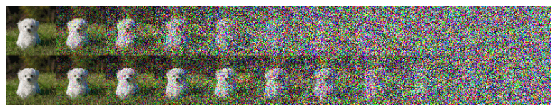
output_img = vae_decoder(latents)

The core idea behind diffusion models is to train a model (called unet above) to predict how to denoise an image. We want to do this in an unsupervised way. So we take normal images, iteratively add gaussian noise to them, and train unet to predict what noise was added. Then, all we have to do when we want to generate an image is: 1) start with random noise, 2) ask our unet for the noise prediction, and 3) iteratively subtract out that noise. The hope is that with this training regime, the unet learns a world model. My goal was to pull out representations from this world model with sparse autoencoders.

The unet is series of convolutions and cross-attention blocks that downsample the spatial dimensions of our latents while increasing their channel dimension and then doing the opposite to get back to the spatial dimensions and channels of the original input. These are called cross-attention blocks because they enable attention across modalities, connecting image latents with text embeddings.

The denoising loop happens over a series of timesteps, and these timesteps are generated via a scheduler. The more timesteps you use, the higher fidelity your image is. There are several schedulers to choose from - each with differing downstream effects on generated images. I used a deterministic scheduler called DDIM in order to have reproducible experiments. The scheduler.step has different algorithms (Runge-Kutta, linear-multistep) to subtract out noise in fancy ways - resulting in an incrementally higher fidelity latents tensor.

Older diffusion pipelines would veer wildly off course during the denoising process, so researchers would use classifiers to help keep them on track. More recently, the field has moved towards using negative prompts, i.e. users can pass in a text prompt of things to avoid. In this "classifier-free guidance", the unet predicts noise for both the positive and negative prompts in parallel. These predictions are then combined using a hyperparameter, G, which linearly interpolates between both noise predictions. Note that if a negative prompt isn't passed to the pipeline, random embeddings are used and denoised. This presents a design decision for us when designing our SAE training pipeline...

Which activations do we train our SAE on?

This section is going to be a discussion on where we should capture diffusion activations from. We have a couple of options:

1. We can try the final activations after all denoising steps.
2. We can try somewhere in the unet, specifically the weights in the cross-attention blocks.

It turns out that 2 is better than 1 because we want to capture A) rich feature representations and B) temporal information.

A) The cross-attention blocks have up to 1,280 channels at each spatial location compared to just four in the final latents. The hypothesis is that concept specialization occurs in different layers or channels.

B) In the denoising loop, there is causal influence over timesteps: Changes in the activations across in earlier timesteps will affect inputs (and therefore outputs) of later timesteps. If we simply train our SAE on the end outputs after all steps, we lose information on this "evolution" of latents.

So we now know that we want latents from the unet across all denoising steps. Where exactly within the unet do we want to sample from? Cywiński & Deja (2025) identified the "up1.1" cross-attention blocks as effective for unlearning via ablation studies. As alluded to above, the unet denoises both pos_noise_pred and neg_noise_pred in parallel. We can actually ignore neg_noise_pred since they represent what the model would generate without any text prompt. The concepts we want to isolate live in the 16x16x1280 shaped activations of the "up1.1" cross-attention block that correspond to pos_noise_pred.

SAE Training Architecture

This brings us to actually training the SAE. This part is relatively straightforward. I have a dataset of 80k prompts that I pass through the diffusion pipeline - collecting activations from the analog of a residual stream of the "up1.1" cross-attention block - and storing them to disk. The activations have a shape of batch * 2, channel, h, w for each step in the denoising pipeline. The first half of the batch dimension corresponds to the negative conditioned activations as described above and the second half correspond to the positive text conditioned activations. We can throw away the negative conditioned activations as described above, stack each timestep, and do a nice rearrange, leaving us with steps * batch, h * w, channel . The resulting activation dataset was ~2.6TB and took ~10hrs to collect.

I wrote a script to chunk files and perform resumable streaming uploads to GCP. Unfortunately, some hidden data egress charges slapped me in the face. In the middle of the upload, the costs ate up my remaining credits and my GPU provider (Vast.ai) killed my instance, destroying all my data. After this experience, I realized it was more cost effective to just train the SAE directly after activation collection on the same GPU.

My training setup heavily referenced Cywiński & Deja (2025). I trained the SAE (expansion_factor=16) for 180k steps which took about 3 hours (wandb). The SAE was a mostly standard architecture, except it used a topk activation - retaining only the k=32 largest SAE latents, and setting the others to zero.

At each training step, I unit-normalize decoder weights for training stability and to improve interpretability and steering of features since they should all be on the same scale. I do this by subtracting out the decoder gradients that are parallel to the existing decoder weights. This leaves us with decoder gradients that are orthogonal to decoder weights, which means the optimizer step will only rotate the weights instead of also scaling them (maintaining their unit norm).

SAE Steering Architecture

There are two steps to steering: 1) calculating feature importances, 2) inferencing the diffusion pipeline with steered activations.

Calculating Feature Importance

Prompts are split into 20 concepts (dogs, cats, trees, etc.) and passed through the diffusion model to collect activations. These activations are passed through the trained SAE encoder and used to calculate feature importances, e.g. which directions in the latent space correspond to each concept. Notably, we calculate feature importances independently for each timestep.

Steering the Generation Process

Let's say we want to steer the generation process to produce fewer guns. First, we would use our precalculated feature importances to find the 99th percentile most activating feature on the gun concept. We then downweight those feature(s) by a factor (γ=20), while leaving the remaining features untouched. We pass this steered SAE latent through the SAE decoder to receive steered diffusion unet activations. These activations are then passed through the remainder of the diffusion pipeline. This happens independently at each denoising timestep, eventually generating a steered image!

Check out the live demo here!

Lessons Learned

Memmaps with pinned memory are great dataset backers

When dealing with massive activation datasets (mine was ~2.6TB), traditional approaches quickly become infeasible. Memory-mapped files (memmaps) provide an elegant solution by creating a mapping between file contents on disk and virtual memory addresses in your process.

Instead of reading the entire dataset into RAM upfront, the OS creates a virtual memory mapping to the file. When your training loop requests a specific batch, the OS loads only those pages from disk into physical memory on-demand.

The magic happens at the page level. Modern operating systems manage memory in 4KB pages, and the memory mapper loads these pages as needed. When you access activations[batch_idx:batch_idx+32], the OS checks if those memory pages are already resident. If not, it triggers a page fault, loads the required pages from disk, and returns control to your program. From your perspective, you're just indexing into a massive array.

Pinned memory takes this a step further by optimizing GPU transfers. Normally, when transferring data from CPU to GPU, the system must first copy from pageable memory to a temporary pinned buffer, then from that buffer to GPU memory - that's two expensive copy operations. With pinned memory, data can be transferred directly from CPU to GPU memory using faster DMA (Direct Memory Access), eliminating the intermediate copy step.

Tuning Parameters for Optimal Loading

Unlike most deep learning regimes, training Sparse Autoencoders from cached activations is dominated by IO latency as opposed to FLOP/S. Therefore, we really want to make sure we have efficient loading from disk. I found through tuning that using num_workers=2 and prefetch_factor=8 achieved the highest throughput within a reasonable max memory usage on an H100.

SSH Sessions are Volatile

I use the remote-ssh extension on Cursor to work on remote GPUs. However, this becomes a problem when the SSH clients on my local machine sleep. I learned this the hard way during my first activation collection run when I woke up to find my long running job had died sometime around 2am.

Running a Python process directly in an SSH session ties that process to the foreground of your session. The moment your SSH connection drops - whether from network issues, laptop sleep, or just closing the terminal - your process gets a SIGHUP signal and dies.

Terminal multiplexers like tmux solve this by creating persistent sessions that live independently of your SSH connection. This lesson applies beyond just SSH volatility - any time you're running expensive compute jobs, you want them decoupled from your interactive session. I'm sure people already know this or use heavier-weight tools like Airflow for job orchestration, but you live and you learn.

Don't Jump OOMS

These are exciting times for machine learning! We have powerful frameworks and tooling that enable us to work with data and compute at Orders of Magnitude more than what was possible just a few years ago - and that with just a few dollars and keystrokes. This kind of power is exhilarating for a newer ML practitioner. There's a tendency towards prototyping and experimenting at large scales. However, fast feedback loops are critical and the tooling doesn't solve all of your problems.

I learned that it's important to have 1-click ways to traverse OOMs. Configuration via arg passing is powerful but not the whole story. I landed on launch configs + makefiles to set batch sizes / expansion factors / parameter counts (which I'll collectively call scale factors here). Spending some time upfront to play with different combinations of hyperparameters + scale factors that get you reasonable performance across OOMs is very important and would have saved me a lot of time. The simplifying principle, I realized, is to debug at the smallest OOM your problem presents itself at.

Also, it's helpful to delineate OOMs in terms of duration of runtimes: 1s, 10s, 1 min, 10 mins, 1 hr, 10hrs - and choose scale factor combos that give you roughly those runtimes. Tensor shape / broadcasting bugs should definitely be handled at 1s runtimes, while disk performance should be iterated on at 10 min runtimes.

Finally, it's tempting to try to find the cheapest hardware that allows you to hit the OOM you're working with at the moment. For example, I spent a lot of time working with RTX 5090s. However, if you can afford it, choose a workhorse GPU (A100 or H100) and use that for everything that needs a GPU. Switching between GPU models makes calculating scale factors annoying (you now have to take into account different FLOPS), but more importantly, different optimizations only work with certain architectures, i.e. Flash Attention 3 is architecture aware and only works on Hopper architectures.

I wish I had spent less time learning how to quickly switch between heterogeneous GPU types and more time simplifying switching between OOMs.

Check out the live demo here!

Next Steps

This project had a few engineering goals:

1. Learn about provisioning and running large machine learning workloads on remote GPUs ✅
2. Learn about training Sparse Autoencoders ✅
3. Demonstrate the usage of SAEs on downstream tasks ✅

In the future, I would love to focus more on scientific experimentation. Anecdotally, we can see that steering on "Bear" features tends to modify face and maw of bears. Could we use spatial maps to help with interpretability of SAE features? Also, it would be fun to experiment with different SAE architectures and their affects on downstream steering tasks.

Acknowledgements

Code and methods adapted from:

• Cywiński, B., & Deja, K. (2025). SAeUron: Interpretable Concept Unlearning in Diffusion Models with Sparse Autoencoders. arXiv:2501.18052v2 [cs.LG].

• Gao, L., Dupré la Tour, T., Tillman, H., Goh, G., Troll, R., Radford, A., Sutskever, I., Leike, J., & Wu, J. (2024). Scaling and evaluating sparse autoencoders. arXiv:2406.04093 [cs.LG].

Dataset Prompt data adapted from:

• Zhang, Y., et al. (2024). UnlearnCanvas: A Stylized Image Dataset for Enhanced Machine Unlearning Evaluation in Diffusion Models.